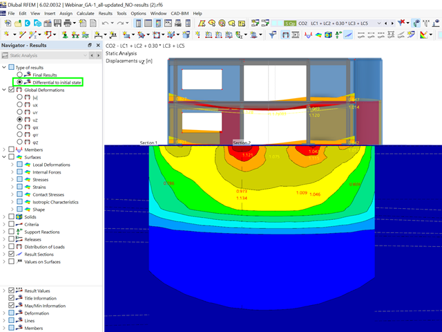
Did you already know? For load combinations, you can optionally display the difference results to the initial state. For example, you have the option for a geotechnical analysis to output the settlement as a difference to the initial state "soil self-weight".
.png?mw=640&hash=55038d2a1591f62179796666cb9b2fede0274e19)
A graphical and tabular output of the results for deformations, stresses, and strains helps you when determining the soil solids. To achieve this, use the special filter criteria for targeted selection of results.
The program doesn't leave you alone with the results. If you want to graphically evaluate the results in the soil solids, you can use the guide objects. For example, you can define clipping planes. This allows you to view the corresponding results in any plane of the soil solid.
And not just that. The utilization of result sections and clipping boxes facilitates the precise graphical analysis of the soil solid.
You already know that it is possible to model and analyze a soil and a structure in the entire model. As a result, you have explicitly taken into account the soil-structure interaction. By modifying a component, you achieve the immediate correct consideration in the analysis as well as in the results for the entire system of the soil and structure.

Are you ready for the evaluation? Use the calculation diagrams, which show the distribution of a specific result during the calculation.
You can freely define the layout of the vertical and horizontal axes of the calculation diagram. This allows you, for example, to consider the settlement distribution of a certain node, depending on the load.

Your data are always documented in a multilingual printout report. You can adjust the content at any time and save it as a template. You can also add graphics, texts, MathML formulas, and PDF documents to your report with just a few clicks.

Enter and model a soil solid directly in RFEM. You can combine the soil material models with all common RFEM add-ons.
This allows you to easily analyze the entire models with a complete representation of the soil-structure interaction.
All parameters required for the calculation are automatically determined from the material data that you have entered. The program then generates the stress-strain curves for each FE element.

Did you know? You can enter the soil layers that you have obtained from the subsoil expertises done in the locations into the program in the form of soil samples. Assign the explored soil materials, including their material properties, to the layers.
For the definition of the samples, you can enter the data in tables as well as in the respective editing dialog box. Furthermore, you can also specify the groundwater level in the soil samples.

The soil solids that you want to analyze are summarized in soil massifs.
Use the soil samples as a basis for a definition of the respective soil massif. This way, the program allows for user-friendly generation of the massif, including the automatic determination of the layer interfaces from the sample data, as well as the groundwater level and the boundary surface supports.
Soil massifs provide you with the option to specify a target FE mesh size independently of the global setting for the rest of the structure. You can thus consider the various requirements of the building and soil in the entire model.

Do you want to model and analyze the behavior of a soil solid? To ensure this, special suitable material models have been implemented in RFEM.
You can use the modified Mohr-Coulomb model with a linear-elastic ideal-plastic model or a nonlinear elastic model with an oedometric stress-strain relation. The limit criterion, which describes the transition from the elastic area to that of the plastic flow, is defined according to Mohr-Coulomb.

Compared to the RF‑SOILIN add-on module (RFEM‑5), the following new features have been added to the Geotechnical Analysis add-on for RFEM 6:
- Creation of the layered soil as a 3D model from the entirety of the defined soil samples
- Recognized material law according to Mohr-Coulomb for soil simulation
- Graphical and tabular output of stresses and strains at any depth of the soil
- Optimal consideration of the soil-structure interaction on the basis of an overall model

- Realistic representation of interaction between a building and soil
- Realistic representation of the influences of the foundation components on each other
- Extensible library of soil properties
- Consideration of several soil samples (probes) at different locations, even outside the building
- Determination of settlements and stress diagrams as well as their graphical and tabular display
Entering soil layers for soil samples is performed in a clearly arranged dialog box. A corresponding graphical representation supports clarity and makes checking the input user-friendly.
An extensible database facilitates the selection of soil material properties. The Mohr-Coulomb model as well as a nonlinear model with stress and strain dependent stiffness are available for a realistic modeling of the soil material behavior.
You can define any number of soil samples and layers. The soil is generated from all entered samples using 3D solids. Assignment to the structure is carried out using coordinates.
The soil body is calculated according to the nonlinear iterative method. The calculated stresses and settlements are displayed graphically and in tables.
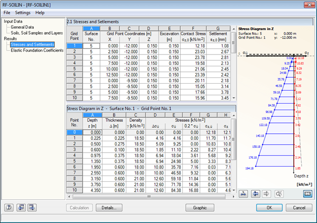
The calculated stresses and settlements are displayed in result windows. In addition, it is possible to evaluate the results graphically. The graphic displays the position and the layer arrangement of the soil samples to clarify the results.
The final result window shows the elastic foundation coefficients. Graphical evaluation is possible as well.
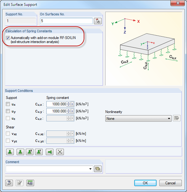
Elastic foundation coefficients are calculated according to the non-linear iterative method. The module determines elastic foundation coefficients for each individual element. They are dependent on the deformation.
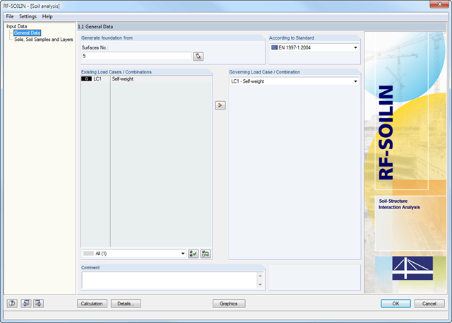
The definition of soil layers is performed in a clearly arranged input window. An extensible library facilitates the selection of soil properties.
The elasticity can be defined either by the stiffness modulus or the modulus of elasticity and the Poisson's ratio. It is possible to define any number of soil layers. You can assign the layers to the building graphically or by entering the relevant coordinates.
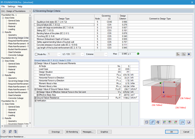
It is possible to perform the following designs:
- Equilibrium limit state design
- Uplift limit state design
- Ground failure (soil contact pressure) design
- Strong eccentric loads design
- Design of foundation torsion and limitation of gaping joint
- Sliding design
- Settlement calculation
- Bending failure design of the plate and bucket
- Punching shear design
Foundation and bucket dimensions can be user-defined or determined by the module. You can edit the determined reinforcement manually. In this case, the designs are updated automatically.
.png?mw=640&hash=34966a7f3c34f6b7bb83003f1c13cb57a2f0cabb)
- Realistic representation of interaction between a building and soil
- Extensible library of soil properties
- Consideration of several soil samples (probes) at different locations, even outside the building
- Consideration of groundwater level as well as side effects due to excavation and lowest soil layer being solid
- Calculation of elastic foundation coefficients
- Determination and graphical display of stress diagrams and settlements in grid points